
Mr Toogood's Physics
A Level Physics notes to support my lessons at LCS
A Level Physics notes to support my lessons at LCS
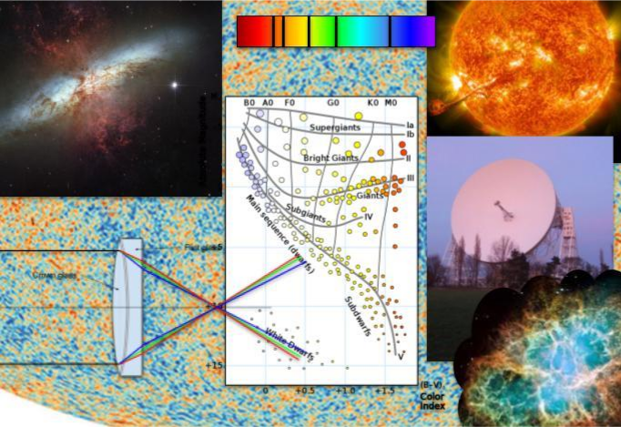
Below you can read exactly what AQA want you to know for this module. You can also find the relevant section from the specification on each page of this site. You should be aware of both what you need to know, and (just as importantly) what you DO NOT need to know. It is also important to remember that you need to be able to apply these statements to a wide range of different contexts, so you must practise this by attempting lots of different questions and reading around the subject.
3.9.1.1 Astronomical telescope consisting of two converging lenses
Ray diagram to show the image formation in normal adjustment.
Angular magnification in normal adjustment.
Focal lengths of the lenses.
3.9.1.2 Reflecting telescopes
Cassegrain arrangement using a parabolic concave primary mirror and convex secondary mirror.
Ray diagram to show path of rays through the telescope up to the eyepiece.
Relative merits of reflectors and refractors including a qualitative treatment of spherical and chromatic aberration.
3.9.1.3 Single dish radio telescopes, I-R, U-V and X-ray telescopes
Similarities and differences of radio telescopes compared to optical telescopes. Discussion should include structure, positioning and use, together with comparisons of resolving and collecting powers.
3.9.1.4 Advantages of large diameter telescopes
Minimum angular resolution of telescope.
Rayleigh criterion,
Collecting power is proportional to diameter2.
Students should be familiar with the rad as the unit of angle.
Comparison of the eye and CCD as detectors in terms of quantum efficiency, resolution, and convenience of use.
No knowledge of the structure of the CCD is required.
3.9.2.1 Classification by luminosity
Apparent magnitude, m.
The Hipparcos scale.
Dimmest visible stars have a magnitude of 6.
Relation between brightness and apparent magnitude. Difference of 1 on magnitude scale is equal to an intensity ratio of 2.51.
Brightness is a subjective scale of measurement.
3.9.2.2 Absolute magnitude, $M$
Parsec and light year.
Definition of M, relation to m:
3.9.2.3 Classification by temperature, black-body radiation
Stefan’s law and Wien’s displacement law.
General shape of black-body curves, use of Wien’s displacement law to estimate black-body temperature of sources.
Experimental verification is not required.
$λ_{max}T = \mathrm{constant}=\\ \quantity{2.9 × 10^{-3}}{m\,K}$
Assumption that a star is a black body.
Inverse square law, assumptions in its application.
Use of Stefan’s law to compare the power output, temperature and size of stars $P=σAT^{4}$
3.9.2.4 Principles of the use of stellar spectral classes
Description of the main classes (see main table)
Temperature related to absorption spectra limited to Hydrogen Balmer absorption lines: requirement for atoms in an $n = 2$ state.
3.9.2.5 The Hertzsprung-Russell (HR) diagram
General shape: main sequence, dwarfs and giants.
Axis scales range from –10 to +15 (absolute magnitude) and $\quantity{50 000}{K}$ to $\quantity{2 500}{K}$ (temperature) or OBAFGKM (spectral class).
Students should be familiar with the position of the Sun on the HR diagram.
Stellar evolution: path of a star similar to our Sun on the HR diagram from formation to white dwarf.
3.9.2.6 Supernovae, neutron stars and black holes
Defining properties: rapid increase in absolute magnitude of supernovae; composition and density of neutron stars; escape velocity $> c$ for black holes.
Gamma ray bursts due to the collapse of supergiant stars to form neutron stars or black holes.
Comparison of energy output with total energy output of the Sun.
Use of type 1a supernovae as standard candles to determine distances. Controversy concerning accelerating Universe and dark energy.
Students should be familiar with the light curve of typical type 1a supernovae.
Supermassive black holes at the centre of galaxies.
Calculation of the radius of the event horizon for a black hole, Schwarzschild radius (Rs),
3.9.3.1 Doppler effect
$\frac{\Delta f}{f}=\frac{v}{c}$ and $z=\frac{\Delta \lambda}{\lambda}=-\frac{v}{c}$ for $v\lt\lt c$ applied to optical and radio frequencies.
Calculations on binary stars viewed in the plane of orbit.
Galaxies and quasars.
3.9.3.2 Hubble's law and the big bang
Red shift $v = Hd$
Simple interpretation as expansion of universe; estimation of age of universe, assuming H is constant.
Qualitative treatment of Big Bang theory including evidence from cosmological microwave background radiation, and relative abundance of hydrogen and helium.
3.9.3.3 Quasars
Quasars as the most distant measurable objects.
Discovery of quasars as bright radio sources.
Quasars show large optical red shifts; estimation involving distance and power output.
Formation of quasars from active supermassive black holes.
3.9.3.4 Detection of exoplanets
Difficulties in the direct detection of exoplanets.
Detection techniques will be limited to variation in Doppler shift (radial velocity method) and the transit method.
Typical light curve.